Show FORMULA or FORMAT of another cell
Location: http://www.mvps.org/dmcritchie/excel/formula.htm
Home page: http://www.mvps.org/dmcritchie/excel/excel.htm
[View without Frames]
[Top]
[GetFormula]
[Install a Macro (moved to another page)]
[GetText]
[GetFormula Example]
[CondFormula]
[GetFormat]
[Ex]
[Custom Number Formatting]
[Comma]
[Fill]
[Debug Format
[Million/Billion]
[Carpentry/Measurement]
[Format/Fill characters]
[HasFormula]
[BoldSum]
[SpecialCells]
[getfontname]
[FontInfo]
[FontStyle]
[Select cells with formulas or constants]
[UseFormula]
[UseSameAs]
[Remove all formulas from a workbook]
[Formula in MsgBox]
[Sheet Statistics]
[More Notes]
[Screen, parts of]
[Status Bar (moved)]
[Large/Small WS Formulas (moved)]
[GetFormulaInfo (moved)]
[AddIn (moved to another page)]
[Troubleshooting]
[Related]
[Bottom]
-- above links should all work even in Firefox, match lettercase shown in your browser's statusbar.
| This page contains some VBA
macros. If you need assistance to install or to use a macro please
refer to my «Getting Started with Macros« or delve into it deeper
on my Install page. |
The formula view is the normal method of showing formulas in Excel, which I find
not very sufficient: (#getformula)
- Tools --> Options --> View --> (formula on/off)
- Ctrl+` is the equivalent shortcut (toggle on/off) -- accent grave to left of the 1,2,3 on the top row
- Also see Select cells with formulas or constants which
you can tab through or use a pattern color to mark the cells.
I prefer to show the formula in use for documentation purposes (see code for GetFormula below),
within the actual spreadsheet they are active in, which I think is the
best choice. Advantage you know
right at that moment you are looking at the content of the formula actually
in use. Since the formula is shown in a regular cell, the
column can be sized appropriately. The formula view shows all formulas
with the columns all proportionally widened about 2 X the normal width.
which is rather arbitrary and any change would affect your normal cell width
so you would want to change column widths on a copy of the file.
The use of GetFormula, I think, is usually much more practical than viewing
a separate list of formulas such as John Walkenbach’s Creating a List of Formulas (Tip 37) mentioned in the Related area.
A simple VBA User Defined Function (UDF) is the solution.
To show the formula of another cell, you can use a simple VBA function.
GetFormula was the first User Defined Function that I wrote following
my first contact with Excel newsgroups. Most of the help came from Alan Beban, who offered me
a more complicated subtroutine with offset. I managed to simplify it by trial and error to exactly what I really wanted in a more generic
formula. It has proven very useful along with the variations listed below it, and
a similar function GetFormat to show number format used.
Specification Limit found in Excel HELP:
Length of cell contents (text) is 32,767 characters. Only 1,024 display in a cell; all 32,767 display in
the formula bar.
(you *may* be able to increase the display with use of Alt+Enter to force a new line}
Length of formula contents is 1,024 characters
The Code for GetFormula
Function GetFormula(Cell as Range) as String
   GetFormula = Cell.Formula
End Function
Usage: Examples using GetFormula
=GetFormula(A1) -- Display the formula used in cell A1
=personal.xls!getformula(A1) -- invoke macro from another workbook
=GetFormula(sheet150!A1) -- get the formula used on another worksheet
=GetFormula('sheet one'!A1) -- other sheetname has spaces
=GetFormula([WBName.xls]WSName!A1) -- from another workbook with caution
Usage in Right Click Menu for faster coding:
Fact is this is one of my most entered formulas, so I added it
to my Right Click Menus
(the regular Context Menus) not to be confused with Event Macros which is another topic.
Variations of the GetFormula User Defined Function:
The following variation might look better but would not match the Formula view of Excel.
Advantage is it shows a single quote if the cell shows up AS TEXT, and it shows array formulas as array formulas with the braces.
Function GetFormulaI(Cell as Range) as String
   'Application.Volatile = True
   If VarType(cell) = 8 And Not cell.HasFormula Then
    GetFormulaI = "'" & cell.Formula
   Else
    GetFormulaI = cell.Formula
   End If
   If cell.HasArray Then _
     GetFormulaI = "{" & cell.Formula & "}"
End Function
The following variation includes the cell address as a descriptor:
Function GetFormulaD(Cell as Range) as String
   GetFormulaD = Cell.Address(0, 0) & ":  " & Cell.Formula
End Function
GetFormulaID is similar to GetFormulaI and GetFormulaID, available
along with other macros on this page -- code for this page.
If you ONLY want to see a formula or nothing. My preference is for GetFormula or GetFormulaI
above but some people ask only to see an actual formula.
I'd rather see what is actually there and besides a constant may not look much
like the formatted text.
Function ShowFormula(Cell as Range) as String
    If cell.HasFormula Then ShowFormula = cell.Formula
End Function
The use of Cell.FormulaLocal in the above functions may work better for non English usage of Excel.
Placing Formulas into Cell Comments is
another approach but would not recommend it as being very practical.
Obtaining intermediate results for a formula is possible but complicated
see GFRV user defined function, posted by Harlan Grove 2002-02-27 misc.
The above functions refer to formula usage (.formula in VBA), a direct assignment
with equal sign can show the value (.value in VBA), the GetText function (below) will
show the text (.text in VBA) result will always be text unless empty or in error.
Reference to an empty cell will result in an empty cell (test for ISBLANK in Excel, ISEMPTY in VBA). A comparable macro can be found in the AllCellsToText macro
on my webpage Proper describing inner workings of some macros, is described as useful in Mail Merge. (similar to another macro As_Text ).
Function GetText(Cell as Range) as String
   On Error Resume Next
   GetText = cell.Text
End Function
Example: (Formula view)
| | A | B | C |
| 1 | =4+5 |
=GetFormula(A1) |
=GetFormula(B1) |
| 2 | =NOW() |
=GetFormula(A2) |
=GetFormula(B2) |
|
|
Example: (Data view)
| | A | B | C |
|---|
| 1 | 9 |
=4+5 |
=GetFormula(A1) |
| 2 | 1/16/98 22:59 |
=Now() |
=GetFormula(A2) |
|
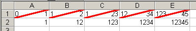
You can copy the =GetFormula(A1) downward to do the column.
Notice that the GetFormula(cellname) also works on GetFormula(cellname).
GetFormula has been very useful for me, hope it helps you as much.
GetFormula failures:
On a protected sheet GetFormula will return #VALUE! if the cell being
examined is hidden. If a cell is hidden you cannot see the formulas
on the formula bar. If a cell is locked you cannot change the
value or formula, but has no effect on GetFormula.
Evaluating A Formula, step by step (#F9)
Highlight a part of the formula in the Formula Bar and press F9.
The highlighted part of the formula is replaced by the result.
If you press Esc then the formula re-appears, but if you press Enter the
formula or part formula is permanently replaced. Charles Williams, 2001-04-20, and then mentions that... In Excel 2002 you can evaluate formulae step by step automatically.
Conditional Formatting is considerably harder to show what you want to see.
It has a range that you can’t just see, anyway the following is a start and will work
best if it just has a formula, rather than “is less than” type of conditions.
Function CondFormula(myCell, Optional cond As Long = 1) As String
  'Bernie Deitrick programming 2000-02-18, modified D.McR 2001-08-07
  Application.Volatile
  CondFormula = myCell.FormatConditions(cond).Formula1
End Function
Install a Macro or User Defined Function (#install)
This topic has been moved to it’s own page install.htm#install
because of it’s length. If you are entirely unfamilar with macros then
please start with Getting Started with Macros and User Defined Functions (UDF).
Excel Add-In .XLA (#addin)
This topic has been moved to another page install.htm#addin
because of it’s length and material that was also moved.
Description information for a Function (#fundesc)
Your User Defined Functions (UDF) can be found using the Paste Function Wizard (Shift + F3).
Select “User Defined” which is near the bottom of the left-hand
window and your UDF will appear on the right-hand window.
This topic has been moved to install.htm#fundesc where
it is covered in more detail.
[Top]
[HasFormula]
[Related]
Another item that I thought would be interesting to document is the cell
formatting string seen below in GetFormat invoking another simple
User Defined Function.
Function GetFormat(Cell as Range) as String
   GetFormat = cell.NumberFormat
End Function
The table below shows examples of both formulas and formats.
Note:
Conditional Formatting can override coloring
of cells including color from normal cell formatting.
=HYPERLINK("http://www.mvps.org/dmcritchie/excel/excel.htm","My Excel Pages")
| |
VALUE |
=GetFormat(A...) |
=GetFormula(A...) |
+ |
| |
A |
B |
C |
D |
|
1 |
17 |
General |
=4+5+8 |
F |
| 2 |
06/25/1998 09:50:55.83 |
mm/dd/yyyy hh:mm:ss.00
US default for =NOW() is m/d/yy h:mm |
=NOW() |
F |
| 2 |
1998-06-25 Thu |
yyyy-mm-dd* ddd
Space fill, left & right justified |
=NOW()
[-- more information on Fill Characters] |
F |
| 3 |
(5,878.00) |
#,##0.00_);[Red](#,##0.00) |
-5878 |
N |
| 4 |
8.89E+10 |
0.00E+00 |
88888888888 |
N |
|
5 |
(212) 555-1212 |
[<=9999999]###-####;(###) ###-#### |
2125551212 |
N |
|
6 |
1.1.4 |
@ |
1.1.4 |
T |
|
7 |
173.23.124.123 |
General |
173.23.124.123 |
T |
|
8 |
123-45-6789 |
000-00-0000 |
123-45-6789 as text or 123456789 as number |
T |
|
9 |
|
General |
|
T |
|
10 |
|
General |
|
O |
|
11 |
Yes |
[Red][>0]"No";[Green]"Yes" |
=-1 |
F |
|
12 |
No |
[Red][>0]"No";[Green]"Yes"
|
=1 |
F |
|
13 |
5.00 |
[Blue][>=5]0.00;[Red][<-2]-0.00;[Yellow]
General;[magenta]"Text:"@
|
=5 |
F |
|
14 |
1.1M |
0.0,,"M"_);(0.0,,"M)";0.0"M"_);@
|
1100000 |
N |
|
15 |
0023 |
0000;(0000);0;@
|
23 |
N |
| 16 |
23 1/2" |
# ??/??\"
|
23.5 |
N |
|
17 |
72° 14' 32" |
[h]° mm' ss\" |
=72.2422 / 24
|
F |
| 18 |
17' 2.4" |
General |
=INT(17.2)&"' "&ROUND(12*MOD(17.2,1),1)&"'" |
F |
| 19 |
17' 2.4" |
General
|
=INT(206.4/12)&"' "&ROUND(MOD(206.4,12),1)&"'" |
F |
| 20 |
17.256 |
0.????_);(0.????);0.????;@
[align on decimal point] |
17.256 |
N |
| 21 |
4 lb. 2.0 oz. |
General |
=INT(4.125)&"lb. "&ROUND(16*MOD(4.125,1),1)&"oz."
|
F |
| 22 |
199 |
General |
=DATEDIF(DATE(1999,6,16),DATE(2000,1,1),"d") |
F |
|
23 |
15 |
General |
=5*ROUNDUP(10.1/5,0) |
F |
|
24 |
My Excel Pages |
General |
=hyperlink("www.mvps.org/dmcritchie/excel/excel.htm","My Excel Pages") |
F |
|
25 |
††††
†††† ††††
|| |
General |
=REPT(REPT(CHAR(134),4)&" ",INT(A1/5))&REPT("|",MOD(A1,5)) See Tally Bar (Five-Bar Gate) |
F |
|
26 |
Begin............... |
@*. |
'Begin [-- more information on Fill Characters] |
T |
|
27 |
.................End |
*.@ |
'End [leader dots, note tab leader dots are not supported] |
T |
|
28 |
12 |
General |
=COUNTA(E15:e26)
(DCOUNT, COUNT, COUNTA, COUNTBLANK,
COUNTIF -- Cell Counting Techniques, J-Walk,
Tip 52) |
T |
|
29 |
63 |
General |
=SUM(D3:D14) |
F |
|
30 |
63 |
General |
=SUM(D3:OFFSET(D15,-1,0)) See reasons to use OFFSET |
F |
|
31 |
6 |
General |
=LARGE('Sheet One'!A14:A19,1)
(Largest number in range) |
F |
|
32 |
15 |
General |
=SUMPRODUCT(LARGE(Sheet1!A14:A19,{1,2,3}))
(Sum of the Largest 3 entries) |
F |
|
33 |
07710-1234 |
[<100000]00000_-_0_0_0_0;
[>0]00000-0000;;@
|
077101234 (5 & 9 digit US zip-codes, and should be left justified) |
N |
|
34 |
222.2E+6 |
##0.0E+0 |
222222222.22
(Engineering notation, powers of 3, posted by Bernard Liengme) |
N |
|
35 |
10 |
General (-10 -15 +10 +20) |
=INDEX(A4:D4,,MATCH(0,A4:D4,1)+1)
(First positive number in a row, posted by Niek Otten +) |
N |
|
36 |
10,000,000 |
#,##0.00_);[Red](#,##0.00)
|
10000000 |
N |
| |
| 37 |
1,00,00,000.00 |
[>=10000000]##\,##\,##\,##0.00;
[>=100000]##\,##\,##0.00;##,##0.00
|
10000000
(This format separates groups for India/Thailand, format valid for
positive numbers up to 99,99,99,999.99 or 999,999,999.99)
in Excel XP see function BhatText as in Thai Bhat currency. =BAHTTEXT(A37)
[Rupees,
Rs., Paise,
lakhs,
crores] == an alternative may be to use
Control Panel, Regional Settings, Numbers, digit grouping.
Negative and Positive Numbers can be handled with
a subroutine or event macro by Norman Harker.
Also see
Rupees & Paise (item #8) by Suresh G. in Office watch. |
N |
+ Column D utilizes the formula shown with
HasFormula in the next topic below.
F=Formula, N=Number, T=Test, O=Other
Additional Examples of Normal Cell formatting can be found on
my Conditional Formatting page.
A9 has a single blank, A10 is an untouched cell will test as ISBLANK (or as ISEMPTY in VBA)
| Format | Formatted | Formatted |
Format you see in Custom (#numberformat) |
| General | 55000 | -4123.44 |
General |
| accounting | $ 55,000.00 |
$ (4,123.44) |
_($* #,##0.00_);_($* (#,##0.00);_($* "-"??_);_(@_) |
| currency | $55,000.00 |
($4,123.44) |
$#,##0.00;[Red]$#,##0.00 |
| number | 55000.00 |
4123.44 |
0.00;[Red]0.00 |
| number | 55,000.00 |
4,123.44 |
#,##0.00;[Red]#,##0.00 |
| Custom | $***55,000.00 |
$****(4,123.44) |
_($**#,##0.00_);[Red]_($**(#,##0.00);_($* "-"??_);_(@_) |
| Custom | ***$55,000.00 |
****$(4,123.44) |
_(**$#,##0.00_);[Red]_(**$(#,##0.00);_(**$0.00_);_(@_) |
The examples with asterisks(*) would be used for check writing protection,
and would probably be combined with spelling out the amount in words
as in Numbers to words on my
Strings page. It should be noted that there
are differences in US and British use of the word AND and you want to choose
how you want the currency and fractional amout to show up. One Example:
One Hundred Eleven Dollars And 11/100
Using Formatting to Change the Way Numbers, Dates, Times, and Text Appear in Microsoft Excel, //dead link//
http://support.microsoft.com/default.aspx?scid=/support/Excel/Content/Formats/default.asp
Custom Cell Formatting (#custom)
For more information on formatting see your Excel HELP. My Formula page has Cell Formatting information.
| -4 |
[>=5]General; [Red]-General; [Blue]General |
| -1 |
[>=5]General; [Red]-General; [Blue]General |
| 0 |
[>=5]General; [Red]-General; [Blue]General |
| 2 |
[>=5]General; [Red]-General; [Blue]General |
| 4 |
[>=5]General; [Red]-General; [Blue]General |
| 5 |
[>=5]General; [Red]-General; [Blue]General |
| 10 |
[>=5]General; [Red]-General; [Blue]General |
| txt | [>=5]General; [Red]-General; [Blue]General |
| |
|
Entry |
Formatted |
Format -- GetFormat(cell) was used to display Format |
| -7 | - 7.00 |
[Blue][>=5]0.00; [Red][<=2]-0.00; [Color 42]General; [magenta]"Text:"@ |
| -3 | - 3.00 |
[Blue][>=5]0.00; [Red][<=2]-0.00; [Color 42]General; [magenta]"Text:"@ |
| -2 | - 2.00 |
[Blue][>=5]0.00; [Red][<=2]-0.00; [Color 42]General; [magenta]"Text:"@ |
| -1 | - 1.00 |
[Blue][>=5]0.00; [Red][<=2]-0.00; [Color 42]General; [magenta]"Text:"@ |
| 0 | 0.00 |
[Blue][>=5]0.00; [Red][<=2]-0.00; [Color 42]General; [magenta]"Text:"@ |
| 1 | 1.00 |
[Blue][>=5]0.00; [Red][<=2]-0.00; [Color 42]General; [magenta]"Text:"@ |
| 2 | 2.00 |
[Blue][>=5]0.00; [Red][<=2]-0.00; [Color 42]General; [magenta]"Text:"@ |
| 3 | 3 |
[Blue][>=5]0.00; [Red][<=2]-0.00; [Color 42]General; [magenta]"Text:"@ |
| 4 | 4 |
[Blue][>=5]0.00; [Red][<=2]-0.00; [Color 42]General; [magenta]"Text:"@ |
| 5 | 5.00 |
[Blue][>=5]0.00; [Red][<=2]-0.00; [Color 42]General; [magenta]"Text:"@ |
| 6 | 6.00 |
[Blue][>=5]0.00; [Red][<=2]-0.00; [Color 42]General; [magenta]"Text:"@ |
| 7 | 7.00 |
[Blue][>=5]0.00; [Red][<=2]-0.00; [Color 42]General; [magenta]"Text:"@ |
| Test | Text:Test |
[Blue][>=5]0.00; [Red][<=2]-0.00; [Color 45]General; [magenta]"Text:"@ |
|
see the topic “Create a custom number format”
in your Excel Help (#syntax)
Format for ... (each format is separated by a semicolon)
Positive Numbers(default); Negative Numbers(default); Zero(All other numbers); Text
|
To color negative numbers RED and other numbers black.
Format --> Cells --> Number --> Custom --> #,##0.00_);[Red](#,##0.00)
The number currently in the cell will be shown for the examples you chose from.
If you wanted to modify that further you may do so all within custom format.
By making the third parameter empty (must be within consecutive semi-colon list separators) you
can selectively suppress zero valued cells when using a format such as:
#,###.00;-#,###.00;;@
This method would generally be preferrable to suppressing zeros via Tools, Options, View, and
unchecking Zero values (applies to the worksheet), and better than using Conditional
Formatting to white out zero values. Use of page setup, sheet, Print B&W
will override attempts to white out with Conditional Formatting. Use of Select ALL (Ctrl+A)
will show values on the screen even though their font is white or effectively white.
To complete hide a cell you can use a format of ;;;; (four list separators).
If you do not find the format you want, choose the format that is closest to
what you want, and then.use custom formatting to modify it to what you want.
For text formatting simply use the toolbar button that looks like a T (for text) with a color block in front -- there is a pull down beside it. There is a similar button with a paint bucket behind the block for background; and another button with a pencil behind it for shading.
Microsoft Office Assistance: Create or delete a custom number format is where you can see the syntax
and other descriptions of number formattig -- but you must use the Show all
or Hide All or topic indicator arrows..
Comma Separator (#comma)
The digit grouping separator in the US is the comma which is used to separate the thousands. If you use another character in the US you will not get the same result, unless extra characters of "0" or "#" are explicitly included in the format. below includes examples attempting to use a space and a hyphen.
| | A | B | C | D | E |
| 1 | -1 |
-1.00 |
(1.00) |
( 1.00) |
(-1.00) |
| 2 | -100 |
-100.00 |
(100.00) |
( 100.00) |
(-100.00) |
| 3 | -10000 |
-10000.00 |
(10,000.00) |
(10 000.00) |
(10-000.00) |
| 4 | -100000 |
-100000.00 |
(100,000.00) |
(100 000.00) |
(100-000.00) |
| 5 | -10000000 |
-10000000.00 |
(10,000,000.00) |
(10000 000.00) |
(10000-000.00) |
| 6 | |
| |
| |
| 7 | 1 |
1.00 | 1.00 |
1.00 | -1.00 |
| 8 | 100 |
100.00 | 100.00 |
100.00 | -100.00 |
| 9 | 10000 |
10000.00 | 10,000.00 |
10 000.00 | 10-000.00 |
| 10 | 100000 |
100000.00 | 100,000.00 |
100 000.00 | 100-000.00 |
| 11 | 10000000 |
10000000.00 | 10,000,000.00 |
10000 000.00 | 10000-000.00 |
| 12 | | | |
| |
| 13 |
General |
0.00 |
#,##0.00_);[Red](#,##0.00) |
|
| 14 | | | |
# ##0.00_);[Red](# ##0.00) |
| 15 | | | |
#-##0.00_);[Red](#-##0.00) |
| |
| | A | B |
| 16 | 33333.55 | General |
| 17 | $33,333.55 |
$#,##0.00 |
| 18 | $*******33,333.55 |
$**#,##0.00 |
| 19 | *******$33,333.55 |
**$#,##0.00 |
| 20 | $ 33.59 |
_($* #,##0.00_);_($* (#,##0.00);_($* "-"??_);_(@_) |
| 21 | 33.6 | General |
|
Fill Characters used in FORMAT ...... (#fill)
Repeating characters To repeat the next character in the format to fill the column width, include an asterisk (*) in the number
format. For example, type 0*- to include enough dashes after a number to fill the cell.
Format --> cells --> custom
     A1:      0*.          number value  1
     A1:      @*.          text value:   '1
     B1:      General      text value:  Monday
     B1:      *.dddd       number   value:  01/31/2000      (US)
There is also format --> cells --> alignment --> horiz. --> fill
which will fill the entire cell with repeated value
Formatting to split a number to left and right of a cell, J.E.McGimpsey,
2004-02-07. (#diagformat)
[<=99]0* 0;[<=999]0* 00;00* 00;@
Format the diagonal line with format, cells, borders.
Finding out what you actually have -- it may not be what it looks like.
Some worksheet formulas to help show what you actually have:
=IF(ISTEXT(E2),"T",IF(ISNUMBER(E2),"N","L"))&LEN(E2)
=ISNUMBER(E2)
=ISTEXT(E2)
=LEN(E2)
=ISBLANK(E2) [in VBA the equivalent is ISEMPTY]
=CODE(E2) =CODE(RIGHT(E2,1)) [in VBA the equivalent is ASC], Chip Pearson's “Cell View” addin makes
viewing code within a cell easier.
=personal.xls!GetFormula(E2)
=personal.xls!GetFormat(E2)
There is no ISDATE function in Excel but you can create your own with
Function isdate(cell) As Boolean
isdate = VBA.isdate(cell)
End Function
Check what the cell was formatted for with Format, cells and look at the
format.
Changing the format between Text and Number (or between Number and Text) will have no effect
on data already entered, but reentry of data will be changed if valid.
Changing the format of a cell does not cause the format to
actually change between text and number or between
number and text. The data has to be reentered.
If the cell was already formatted as a number and that format was
in effect then you can change to another number format and it will
be immediately effective.
Changing the number format for a cell that is a number, shows true for
=ISNUMBER(C2), will be immediately effective when the format is changed.
The CODE Worksheet Function determines the ASCII code for a single character.
The TRIM Worksheet Function will remove code 32 space from left and right sides.
But a macro such as TRIMALL can simply the TRIM by doing it in place and by converting the HTML (non-breaking space) character 160 to spaaces before trimming.
The formula or text may be reentered by hitting F2 (activate cell and formula bar) then Enter, which is fine for
individual cells. Another manual technique is the Replace (Ctrl+H)
all equal signs (=) by equal signs. Hitting F9 (Recalculate) will cause a reevaluation
based on what is left, if done from the formula bar with highlighted text.
For some macros to effect a Replace see my page on reformatting look for reenter
Colors: black, blue, green, cyan, red, magenta, yellow, white, color1, ..., color56.
See Colors for additional
Color formatting examples.
72° 14' 32" -- Displaying Latitude & Longitude, code as time by dividing decimal degrees by 24 to appear as hours, and format the cell as [h]° mm' ss\" under Format|Custom where the degree symbol is typed ALT+0176 on the numeric keypad. For formatting a temperature: #"°F" More information on these and other symbols including a link to to
a spreadsheet for nautical navigation. [also see Latitude on xlindex page]
A text version formula has similar looking results, but can no longer be treated as a number.
=INT(72.2422 )&CHAR(176)&" " & TEXT( (72.2422 -INT(72.2422 ))*60,"#0.00") &CHAR(146)
Note: 0176 is the degree symbol, 0186 looks similar is actually a superscript zero and is a little larger.
One way to simplify creating custom formats is to pick the best match say
under number or fractions. Then keeping the same cell selected go to custom
format. Also in custom note that as you change the formatting the example will change.
Parenthesis [or brackets] for negative numbers are not equally
available in all language versions of Excel. To get the parens where
not supported directly, change in Control Panel, Regional Settings, Accounting Tab. The latter
does let me select negative figures in brackets. [Jim Rech 2002-07-16, and continues]
Curiously enough you have to make this change on the currency tab in Control
Panel. After doing so the option to have negatives in parens will appear in
Format, Cells, Number, Number, Negative numbers list box. You can always
use a custom number format to get there too, but I know it is convenient to
pick this format from a list. [Jim Rech]
To provide blanks to right of numbers use two underscores. The first underscore indicates to copy the next character as is, while the second underscore will actually be a blank. Notice the ?? used in fractions can also be used to align decimal points in numbers like 129.43 and 10.125
| | A | B | C | D | E |
| 23 | Description |
Feet | Inches | Format |
Format |
| 24 | Descript 1 | 5' |
11" | #'__ | General\" |
| 25 | Descript 2 | 55' |
11.5" | #'__ | General\" |
| 26 | Total |
61' | 0.875" | #'__ | General\" |
| 27 | | |
| | |
| 28 | | Cell |
Formulas used |
| 29 | | B26: |
=INT(SUM(B24:B25)+SUM(C24:C25)/12) |
| 30 | | C26: |
=MOD(SUM(B24:B25)+SUM(C24:C25)/12,1) |
The inches are numeric but formatted Left above
Rounding (#round)
Rounding up to nearest one half
=INT(ROUND((A1+0.5)/0.5,1))*0.5
Conversion -- Millions, Billions (#convertmb)
Data represented as 1.9B, 10.7B, 138.4B, 14.2B, 2.3B, 247.0M, etc.
Note the 'B' is billions and 'M' is millions needs to be converted
to numbers for sorting.
Do a find and replace, and replace B with E9, then replace M with E6.
Billions are 10^9 or 1E9, and Millions are 10^6 or 1E6. This converts the
non-numbers into numbers. Jon Peltier, misc,
2002-06-22
Carpentry, and measurements in Feet and Inches (#carpentry)
This formula from a posting by Bernie Dietrick 2000-08-04 will round to the
nearest 16 inch.
Conversions of Feet and Inches, decimal to 1/16th inch fractional measurements
| Feet | Carpentry |
| 1.2 | 1' - 2 3/8" |
| 1.3333 | 1' - 4" |
| 0.66665 | - 8" |
| 1.0056 |
1' - 0 1/16" |
| 283.065 |
283' - 0 3/4" |
| |
This formula from a posting by Bernie Dietrick 2000-08-04 will round feet and decimal feet to feet, inches with
rounded 1/16 inch fractions.
(also see «
Fractions rounded to 1/4, 1/8, 1/16, 1/32, 1/64, and 1/128)
=IF(A1>=1,INT(A1)&"' ","") & TEXT(MOD(A1,1)*12,"-
0"&IF(ABS(MOD(A1,1)*12-ROUND(MOD(A1,1)*12,0))>1/32,"
0/"&CHOOSE(ROUND(MOD(MOD(A1,1)*12,1)*16,0),16,8,16,4,16,8,16,2,16,8,16,4,16,8,16),""))
&""""
|
Bernie also supplied version from inches with decimal fractions to feet and inches with
rounded 1/16th inch fractions.
=INT(A1/12)&"' " &
TEXT(MOD(A1,12),"0"&IF(ABS(MOD(A1,12)-ROUND(MOD(A1,12),0))>1/32,"
0/"&CHOOSE(ROUND(MOD(MOD(A1,12),1)*16,0),16,8,16,4,16,8,16,2,16,8,16,4,16,8,
16),"")) & """"
and a version from inches with decimal fractions to inches only with rounded 1/16th inch fractions.
=TEXT(A1,"0"&IF(ABS(A1-ROUND(A1,0))>1/32,"
0/"&CHOOSE(ROUND(MOD(A1,1)*16,0),16,8,16,4,16,8,16,2,16,8,16,4,16,8,16),""))
&""""
and a formula to take Feet and Inches back to a number of feet (Bernie Deitrick)
=VALUE(LEFT(A1,FIND("'",A1)-1)) +
VALUE(MID(A1,FIND("'",A1)+1,FIND("""",A1)-FIND("'",A1)-1))/12
or a formula to take Feet and Inches back to a number of inches (based on Bernie Deitrick’s previous solution)
=VALUE(LEFT(A1,FIND("'",A1)-1))*12 + VALUE(MID(A1,FIND("'",A1)+1,FIND("""",A1)-FIND("'",A1)-1))
For those doing carpentry or other things that require trying to get the most
pieces cut from sheet stock (plywood) or linear stock (pipe, and 2x4s) see
Sheet Layout & Lineal Layout in Wood Online Magazine software (pay for), produces a layout and a cut-sheet
list of parts. identified by Gord Dibben don’t know if anyone here has used it.
Additional Worksheet Formulas
created by Bernie Deitrick « for
Fractions rounded to 1/4, 1/8, 1/16, 1/32, 1/64, and 1/128
HasFormula may be used to obtain whether a referenced cell has a formula or not. Actually it works on a range and returns "True" if a formula, "False" if it doesn’t and
#VALUE! if the range has a mixture of the two. HasFormula may help fill in
for some of the information not included with GetFormula. HasFormula was created using a suggestion 06/04/1998 by Nick Manton (nickm@sri.com).
Function HasFormula(cell)
  HasFormula = cell.HasFormula
End Function
Usage: (showing Formula, Number, Text or Other)
=IF(HasFormula(A1),"F",IF(ISNUMBER(A1),"N",IF(ISTEXT(A1),"T","O")))
A similar VBA function combining features of both of the above can be found on
John Walkenbach’s site “
Determining the Data Type of a Cell (tip 52)”. Keep in mind that
the returned attribute may not be mutually exclusive to other attributes.
HasFormula can be used directly with Conditional Formatting to indicate cells
that have formulas because it returns True or False which is what
you need for Conditional Formatting.
Alternatives: If you just want to identify cells that have
formulas you use Edit, GoTo (Ctrl+G), Special, Formulas, ...
The VBA equivalent is use of Special Cells,
also see GoTo example below that.
The antithesis of HasFormula, this is specifically designed for use
in a Conditional Formula, if you can't use the worksheet solution Get.Cell
described on page on Conditional Formatting.
Function cf_NotFormula(cell)
   'based on http://www.mvps.org/dmcritchie/excel/formula.htm#HasFormula
   cf_NotFormula = Not cell.HasFormula And Not IsEmpty(cell) _
      And Not cell.Row = 1
End Function
[Top]
[UseFormula]
[Related]
BoldSum, Sum the cells having Bold format attribute (#boldsum)
Function BoldSum(rngCells As Range) As Double
    'BoldSum is recalculated when any value on sheet changes
    Application.Volatile
    Dim cell As Range
    BoldSum = 0
    On Error Resume Next
    For Each cell In rngCells
       If cell.font.Bold Then BoldSum = BoldSum + cell.Value
    Next cell
End Function
A similar
function BoldCnt can be patterned on the above using BoldCnt + 1
A subroutine providing more information than FontStyle immediately below can be found in FormulaBox providing font information about the first cell in a range plus more general information for the other cells in a selection, and
in GetFontName and in FontInfo providing font information for another cell.
Function FontStyle(cell)
    'Won't change value until some value on sheet changes
    Application.Volatile
    FontStyle = cell.font.fontstyle
End Function
[Top]
[UseFormula]
[Related]
How to select Cells with formulas using VBA (#xlcelltypes)
The following which selects cells with constants is derived directly from a
posting by Tom Ogilvy (1999-02-23). Slight modification will make display
be formulas instead. You can quickly tab around the selected cells using
the tab key. Also see cell.HasFormula
and addition information
in the descriptive information on my Proper page.
In VBA
cells.SpecialCells(xlCellTypeConstants).Select 'In Excel 97
cells.SpecialCells(xlConstants).Select 'In Excel 5/95/97
Had you started with a range instead of a single cell you would have selected
from the range rather than from the entire sheet. (a single cell selection
would by default include the current region, which is not necessarily the entire sheet)
The following will color font red for all cells with formulas in the selected range, or
for the current region (Ctrl+Shift+*) if only a single cell is selected. By using Ctrl+A first to select all cells you could include
the entire sheet in the selection, unless you have Excel 2003. If you are
unfortunate to have Excel 2003 you can restore the widely accepted usage of selecting all cells with a macro solution. SpecialCells always applies only to the usedrange, and formulas are always in the used range.
    Sub ColorFormulas()    'xl97 up use xlcelltypeformulas
      Selection.SpecialCells(xlFormulas).Font.ColorIndex = 3
    End Sub
The manual equivalent using Go To under Edit (There is an example
of GoTo in the next topic}
Select a single cell, then Edit=>GoTo=>Special and pick constants, then OK. Please note that the options under formulas are also the options under Constants -- this is not very apparent.
If you wanted formula cells you would select formulas and each of the options under formulas.
With only the formula cells selected you can then use the TAB key to visit each cell with a formula
and can look at the formula used by looking at the formula bar.
Formulas would be xlFormulas or xlCellTypeFormulas depending on your version. Some other cell types in D10SE697 -- SpecialCells Method (gone, see information in HELP, below). Also see notations and use of SpecialCells on my webpage
“Proper, and other Text changes -- Use of SpecialCells”.
SpecialCells Method
F1 (HELP) --> Index --> SpecialCells Method (listed under notations)
Returns a Range object that represents all the cells that match the specified type and value.
Syntax
expression.SpecialCells(Type, Value)
expression Required. An expression that returns a Range object.
Type Required Long. The cells to include. Can be one of the following XlCellType constants.
| Constant | Description |
| xlCellTypeAllFormatConditions | Cells of any format |
| xlCellTypeAllValidation | Cells having validation criteria |
| xlCellTypeBlanks | Empty cells |
| xlCellTypeComments | Cells containing notes |
| xlCellTypeConstants | Cells containing constants |
| xlCellTypeFormulas | Cells containing formulas |
| xlCellTypeLastCell | The last cell in the used range |
| xlCellTypeSameFormatConditions | Cells having the same format |
| xlCellTypeSameValidation Cells | having the same validation criteria |
| xlCellTypeVisible | All visible cells |
Prior to XL97 the Constants did not include CellType in their naming.
Value Variant.
If Type
is either xlCellTypeConstants
or xlCellTypeFormulas,
this argument is used to determine which types of cells to include in
the result. These values can be added together to return more than one
type. The default is to select all constants or formulas, no matter
what the type. Can be one of the following:
xlErrors,
xlLogical,
xlNumbers,
xlTextValues
How to make Cells with formulas stand out -- Manually (#GoTo)
As just indicated: using Go To (Shortcuts to GoTo are Ctrl+G or F5)
Select a single cell, then Edit=>Goto=>Special and then
pick formulas and then OK.
Then use shading cell or color text with the either of those buttons, or using format menu.
Again, had you started with a range instead of a single cell you would have selected from the range rather than from the entire sheet.
| |
| | A | B | C | D |
| 1 |
A1 |
B1 |
C1 |
D1 |
| 2 |
A2 |
B2 |
C2 |
D2 |
| 3 |
A3 |
A3 |
A3 |
D3 |
| 4 |
A4 |
A3 |
A3 |
D4 |
| 5 |
A5 |
B5 |
C5 |
D5 |
|
For presentation purposes. Since this will purposely destroy
all formulas in a workbook ou would only want to run this on a copy
of a live workbook.
Sub Remove_All_Formulas_In_All_Sheets  'No_formula_Macro()
  'Goodnight  2000-10-27 programming -- Striping a workbook of formulas
  Dim SH As Worksheet
  For Each SH In Worksheets
    SH.Activate
    Application.ScreenUpdating = False
    Cells.Select
    Selection.Copy
    Selection.PasteSpecial Paste:=xlValues, Operation:=xlNone, _
      SkipBlanks:= False, Transpose:=False
  Next
End Sub
Replace Formulas having External Links with their Values (#values)
External Links can be identified and removed with Bill Manville’s FindLink
program. Look on xlindex page for additional references
such as John Walkenbach’s Tip #54.
Replacing formulas with external links with their values
similar to copy, and paste special, values. This solution
by Tom Ogilvy 2001-07-27 in programming.
Sub Tester3()
Dim cell As Range
For Each cell In ActiveSheet.UsedRange.SpecialCells(xlFormulas)
  If InStr(cell.Formula, "[") Then
    cell.Formula = cell.Value
  End If
Next
End Sub
If you have Left brackets in any other formulas, then they will also be
changed - but a link to an external workbook should contain a Left bracket.
Could include cells with HYPERLINK worksheet formulas for instance.
You will get an error if there are no cells with formulas on the worksheet.
Also see Convert all cells to text values into
new worksheet.
UseFormula is the opposite of GetFormula. UseFormula will do the calculation based on a formula in the referenced cell, which should be entered as a formula after a single quote making it a text string. The use of UseFormula will be tricky at best so I do not recommend general use of this user defined function. GetFormula is a reliable indicator of a working formula; whereas the use of UseFormula referencing blank, null or invalid formulas will result in errors.
Function UseFormula(cell)
    '-- Usage: Not recommended, see notes
    UseFormula = Application.Evaluate(cell.formula)
End Function
| Literal with formula |
=UseFormula(A1) |
| '=3+4 | 7 |
As previously stated I prefer to use GetFormula for documentation
purposes because
you know you are working with valid formulas that way.
The following attempts to make some limited checks for validity
by checking that the formula begins with an
equal sign, and will not display if the source cell appears
to be blank.
Function UseFormula2(cell)
   'Documented in  http://www.mvps.org/dmcritchie/excel/formula.htm
   ' UseFormula Jul 20, 1998,  UseFormula2 Jun 13, 2000
   'Application.Volatile = True  -- DO NOT DO THIS
    If Trim(cell.Value) = "" Then
       UseFormula2 = ""
       Exit Function
    ElseIf Left(cell.Value, 1) = "=" Then
       UseFormula2 = Application.Evaluate(cell.Formula)
       Exit Function
    Else
       UseFormula2 = "'#bad formula"
    End If
End Function
UseSameAs (#usesameas)
UseSameAs will use the same Formula or Constant as used in the referenced cell of another worksheet. Use of parent as the range object makes formula apply to the sheet that the UseSameAs user defined function.
Function UseSameAs(cell As Range)
   '-- Use the same Formula as used in the referenced cell
   '-- http://mvps.org/dmcritchie/excel/formula.htm#usesameas  2005-09-03 .excel
      Application.Volatile
      If cell.HasFormula Then
        UseSameAs = Application.Caller.Parent.Evaluate(cell.Formula)
      Else   '-- needed if constant looks like a cell address
        UseSameAs = cell.Value
      End If
End Function

sheet1!B4:  77
sheet1!C4:  =5*B4      [displays 385]
sheet2!B4:  88
sheet2!C4:  =personal.xls!UseSameAs(sheet1!B4)    [displays 440]
Something similar in pasting the formula used in another cell
can be seen in a user defined constext menu item see paste.htm#formulas
Note: Use of ROW() ro COLUMN() in the formula will be evaluated
as the row or column of the active cell when last calculated (F9), similar to
crippled use of CELL worksheet Function without a reference cell.
You can reference the cell the formula is in B2:&nhsp;=ROW(B2)
FormulaBox will assist in looking at a few formulas. You can usually obtain information for at least three cells. There is no way of predicting how many cells of your selected range will be shown. There are limits to the size of the textbox but what is shown appears to be a lot less than 1024 bytes. Putting together parts of code form the GetFormulaI and GetFormat we create FormulaBox below, which should prove a lot more practical than repeatedly using Format --> Cells to find the format.
Number, Accounting, Social Security, Phone Number
| FormulaBox: formula & formats |
First Character of (345) is = CHR(0051) or Hex=x'33'
Arial 12 Bold

G28: 345
  General
G29: =D26+D27
  _(* #,##0.00_);_(* (#,##0.00);_(* "-"??_);_(@_)
G30: 188121234
  000-00-0000
G31: 7777777777
  [<=9999999]###-####;(###) ###-####
[OK]>
|
Caution: The results may be truncated, you may not see the full range
of the cells selected, and the last line you see may also be
truncated.
Under XL2000 didn’t see truncation as in XL95,
but there is a less severe limitation
in that the msgbox is not scrollable
and you must use the close [X] button. |
|
Sub FormulaBox()
  'David McRitchie  1998-08-12 1999-08-17
  '  http://www.mvps.org/dmcritchie/excel/excel.htm
  'Place material into MsgBox    [ctrl+n]
  'Will process ranges of one or more columns
  'Application.ScreenUpdating = False
  Dim MsgBoxx As String
  MsgBoxx = "First Character of (" _
    & ActiveCell.Value & ") is " & "=CHR(" _
    & Right("0000" & Asc(ActiveCell.Value), 4) & ") or Hex=x'" _
    & Hex(Asc(ActiveCell.Value)) & "'" & Chr(10) _
    & ActiveCell.Font.Name & " " & ActiveCell.Font.Size _
    & "  " & ActiveCell.Font.FontStyle _
    & Chr(10) & Chr(10)

  For ix = 1 To Selection.Count
      'Selection.Item(ix).NoteText _ ...
      vGetFormulaI = ""
      If VarType(Selection.Item(ix)) = 8 Then
       vGetFormulaI = "'" & Selection.Item(ix).Formula
      Else
       vGetFormulaI = Selection.Item(ix).Formula
      End If
      If Selection.Item(ix).HasArray Then _
        vGetFormulaI = "{" & Selection.Item(ix).Formula & "}"

      'include below if VarType wanted -- don't include for distribution
      '   & " " & VarType(Selection.Item(ix)) _ ..
      MsgBoxx = MsgBoxx _
        & Selection.Item(ix).Address(0, 0) _
        & ": " & vGetFormulaI _
        & Chr(10) & "    " & Selection.Item(ix).NumberFormat & Chr(10)

  Next
  MsgBoxx = MsgBoxx & Chr(10) & "***" 'to verify you've  seen everything
  xyx = MsgBox(MsgBoxx, , "FormulaBox: Formula & Format & " _
      & "Text for " & Selection.Count & " selected cells")
  'Application.ScreenUpdating = True
End Sub
Place comment cells for cells that have a value.
Sub CommentThem()
  Dim cell As Range
  On Error Resume Next
  Selection.ClearComments
  On Error GoTo 0
  For Each cell In Intersect(Selection, ActiveSheet.UsedRange)
     If cell.Formula <> "" Then
        cell.AddComment
        cell.Comment.Visible = False
        On Error Resume Next  'fails on invalid formula
        cell.Comment.Text Text:=cell.Address(0, 0) & _
           "  value:    " & cell.Value & Chr(10) & _
           "  format:   " & cell.NumberFormat & Chr(10) & _
           "  Formula:  " & cell.Formula
        On Error GoTo 0
     End If
  Next cell
End Sub
Display Sheet Statistics (#MsgSheetStats")
|
SheetStats provides sheet statistics in a MsgBox. The following code is modified
from a posting by Tom Ogilvy
Tom Ogilvy is a frequent poster to the
Excel Newsgroups.
| |
| SheetStats for Sheet2 in D:\DIR1\excel\testing.xls |
  Address:      $A$1:$G$13
  Last Row:     13
  Last Column:  7
  Total Cells:  91
    Formulas:   4
    Blanks:     77
    Constants:  10
  Errors:       0
  Logical:      0
  Text:         9
  Numbers:      1
[OK]
|
|
Sub SheetStats()
'Tom Ogilvy  1999-02-24 Tues   excel programming
'Note in XL97 and above xlcelltypeconstants and xlcelltypeformula
Set rng1 = ActiveSheet.UsedRange
On Error Resume Next
numConstants = rng1.SpecialCells(xlConstants).Count
If Err <> 0 Then numConstants = 0: Err = 0
numerrors = rng1.SpecialCells(xlConstants, xlErrors).Count
If Err <> 0 Then numerrors = 0: Err = 0
numLogical = rng1.SpecialCells(xlConstants, xlLogical).Count
If Err <> 0 Then numLogical = 0: Err = 0
numText = rng1.SpecialCells(xlConstants, xlTextValues).Count
If Err <> 0 Then numText = 0: Err = 0
numNumbers = rng1.SpecialCells(xlConstants, xlNumbers).Count
If Err <> 0 Then numNumbers = 0: Err = 0
numformulas = rng1.SpecialCells(xlFormulas).Count
If Err <> 0 Then numformulas = 0: Err = 0
numBlanks = rng1.SpecialCells(xlBlanks).Count
If Err <> 0 Then numBlanks = 0: Err = 0

Msg = "Address:     " & Chr(9) & rng1.Address & Chr(10) & _
      "Last Row:    " & Chr(9) & rng1.Rows(rng1.Rows.Count).Row & Chr(10) & _
      "Last Column: " & Chr(9) & rng1.Columns(rng1.Columns.Count).Column & Chr(10) & _
      "Total Cells: " & Chr(9) & rng1.Count & Chr(10) & _
      "   Formulas: " & Chr(9) & numformulas & Chr(10) & _
      "   Blanks:   " & Chr(9) & numBlanks & Chr(10) & _
      "   Constants:" & Chr(9) & numConstants & Chr(10)

Mg2 = "Errors:      " & Chr(9) & numerrors & Chr(10) & _
      "Logical:     " & Chr(9) & numLogical & Chr(10) & _
      "Text:        " & Chr(9) & numText & Chr(10) & _
      "Numbers:     " & Chr(9) & numNumbers

 title1 = "SheetStats for " & Application.ActiveSheet.Name & _
      " in " & Application.ActiveWorkbook.FullName

 iANS = MsgBox(Msg & Mg2, , title1)

End Sub
Some additional related code:
   MsgBox _
      "Address:     " & Chr(9) & _
          Selection.Address & Chr(10) & _
      "First Cell:    " & Chr(9) & _
          Selection(1).Address & Chr(10) & _
      "Active Cell: " & Chr(9) & _
          ActiveCell.Address & Chr(10) & _
      "Last Cell:    " & Chr(9) & _
          Selection(Selection.Cells.Count).Address & Chr(10)

    'This really doesn't do anything, it might change activecell.
    'Just demos getting and selecting a range
    Dim strt As Range, eend As Range
    Set strt = Selection.Cells(1)
    Set eend = Selection(Selection.Cells.Count)
    Range(strt, eend).Select
GetFontName (#getfontname)
Function getFontName(cell As Range) As String
   getFontName = cell.Font.Name  'D.McR  formula.htm
End Function
FontInfo -- a Function to get font information (#fontinfo)
The default font is identified with Tools, Options, General, Standard Font:
Function fontinfo(cell As Range) As String
  fontinfo = cell.FONT.Name & " -- " & cell.FONT.Size
  If Left(cell.FONT.FontStyle, 7) = "Regular" Then
     fontinfo = Trim(fontinfo & Mid(cell.FONT.FontStyle, 8, 100))
  Else
     fontinfo = Trim(fontinfo & " " & cell.FONT.FontStyle)
  End If
End Function
See my Symbols page.
| |
A |
B |
C |
D |
E |
F |
G |
H |
I |
J |
K |
L |
M |
N |
O |
P |
Q |
R |
| 1 |
|
|
=FontInfo(C3)
|
| 2 |
32 |
|
|
! |
" |
# |
$ |
% |
& |
' |
( |
) |
* |
+ |
, |
- |
. |
/ |
| 3 |
48 |
|
0 |
1 |
2 |
3 |
4 |
5 |
6 |
7 |
8 |
9 |
: |
; |
< |
= |
> |
? |
| 4 |
64 |
|
@ |
A |
B |
C |
D |
E |
F |
G |
H |
I |
J |
K |
L |
M |
N |
O |
| 5 |
80 |
|
P |
Q |
R |
S |
T |
U |
V |
W |
X |
Y |
Z |
[ |
\ |
] |
^ |
_ |
| 6 |
96 |
|
` |
a |
b |
c |
d |
e |
f |
g |
h |
i |
j |
k |
l |
m |
n |
o |
| 7 |
112 |
|
p |
q |
r |
s |
t |
u |
v |
w |
x |
y |
z |
{ |
| |
} |
~ |
|
| 8 |
128 |
|
€ |
|
‚ |
ƒ |
„ |
… |
† |
‡ |
ˆ |
‰ |
Š |
‹ |
Π|
|
Ž |
|
| 9 |
144 |
|
|
‘ |
’ |
“ |
” |
• |
– |
— |
˜ |
™ |
š |
› |
œ |
|
ž |
Ÿ |
| 10 |
160 |
|
|
¡ |
¢ |
£ |
¤ |
¥ |
¦ |
§ |
¨ |
© |
ª |
« |
¬ |
|
® |
¯ |
| 11 |
176 |
|
° |
± |
² |
³ |
´ |
µ |
¶ |
· |
¸ |
¹ |
º |
» |
¼ |
½ |
¾ |
¿ |
| 12 |
192 |
|
À |
Á |
 |
à |
Ä |
Å |
Æ |
Ç |
È |
É |
Ê |
Ë |
Ì |
Í |
Î |
Ï |
| 13 |
208 |
|
Ð |
Ñ |
Ò |
Ó |
Ô |
Õ |
Ö |
× |
Ø |
Ù |
Ú |
Û |
Ü |
Ý |
Þ |
ß |
| 14 |
224 |
|
à |
á |
â |
ã |
ä |
å |
æ |
ç |
è |
é |
ê |
ë |
ì |
í |
î |
ï |
| 15 |
240 |
|
ð |
ñ |
ò |
ó |
ô |
õ |
ö |
÷ |
ø |
ù |
ú |
û |
ü |
ý |
þ |
|
An example of use, depending on what font you actually used in your table the
formula shown might be substituted by something such as:
Arial -- 12 Bold
Webdings -- 12
Wingdings 2 -- 12
A table such as the following can be created using
  C2: =CHAR(32)      D2:  =CHAR(32+1)
  C3: =CHAR(32+16)   D3:  =CHAR(32+17)
The table at the right is for Windows characters, if you want to see what
the equivalent characters would be for HTML with UNIX see
(Table has been modified to use HTML tokens, your results may still
vary depending on your fonts, your system, and your browser)
- References in this document
- BoldSum, Sum the cells having Bold format attribute
FontStyle, Display Font Style used in referenced cell
FormulaBox font information for first cell, and general information for all cells in a selection
- References in other pages on this site
- FONT, test for BOLD with ISBOLD(cell) UDF.
- FONTINFO macro on Formula page.
- Fonts, Getting a List of Installed Fonts (tip 79) -- John Walkenbach (tip 79)
-
A simple technique (for Excel 97 or later) to retrieve a list of installed font names,
and an alternative to an API function on Stephen Bullen’s site for those who don’t have
XL97.
- The Font Thing
-- Sue Fisher [update notes], thanks
to Jim Rech (2000-03-15) for telling us.
- Provides information on installed and uninstalled fonts, font samples for your text, including use of two fonts in samples.
The macro code can be found with the other
code associated with the page.
The concept is based on John Walkenbach's Tip 37 which is formulas only
(see note in related area). Following is a bad example as dates in B & C were populated with a macro.
| | A | B | C | D |
| 1 |
2005-11-06 Sun |
2005-11-07 Mon |
2005-11-07 Mon | 1 |
| 2 |
2005-11-07 Mon |
2005-11-07 Mon |
2005-11-07 Mon | 2 |
| 3 |
2005-11-08 Tue |
2005-11-07 Mon |
2005-11-07 Mon | 3 |
| 4 |
2005-11-09 Wed |
2005-11-07 Mon |
2005-11-07 Mon | 4 |
| 5 |
2005-11-10 Thu |
2005-11-07 Mon |
2005-11-07 Mon | 5 |
| 6 |
2005-11-11 Fri |
2005-11-07 Mon |
2005-11-07 Mon | 6 |
| 7 |
2005-11-12 Sat |
2005-11-07 Mon |
2005-11-07 Mon | 7 |
| 8 |
2005-11-13 Sun | 2005-11-14 Mon |
2005-11-14 Mon | 1 |
| 9 |
2005-11-14 Mon | 2005-11-14 Mon |
2005-11-14 Mon | 2 |
| 10 |
2005-11-15 Tue | 2005-11-14 Mon |
2005-11-14 Mon | 3 |
| |
FormulaSheet Macro Results
| Cell | Text | Value |
Formula | NumberFormat |
| A1 | 2005-11-06 Sun | 2005-11-06 |
38662 | yyyy/mm/dd* ddd |
| B1 | 2005-11-07 Mon | 2005-11-07 |
38663 | yyyy/mm/dd* ddd |
| C1 | 2005-11-07 Mon | 2005-11-07 |
38663 | yyyy/mm/dd* ddd |
| D1 | 1 | 1 |
=WEEKDAY(A1) | General |
| A2 | 2005-11-07 Mon | 2005-11-07 |
38663 | yyyy/mm/dd* ddd |
| B2 | 2005-11-07 Mon | 2005-11-07 |
38663 | yyyy/mm/dd* ddd |
| C2 | 2005-11-07 Mon | 2005-11-07 |
38663 | yyyy/mm/dd* ddd |
| D2 | 2 | 2 |
=WEEKDAY(A2) | General |
|
Some Additional Notes on VBA Usage (#morenotes)
Worksheet Functions used in VBA
F1 (Help) --> answer wizard --> worksheetfunction
Using Microsoft Excel Worksheet Functions in Visual Basic
List of Worksheet Functions Available to Visual Basic
WorksheetFunction Property Example
Didn’t know it but there is a difference between newer usage of
application.worksheetfunction.function and application.function
-- worksheetfunction tells VBA to trap the error. (Chip Pearson, programming,
2003-11-12)
This example displays the result of applying the Min worksheet function to the range A1:A10.
Set myRange = Worksheets("Sheet1").Range("A1:C10")
answer = Application.WorksheetFunction.Min(myRange)
MsgBox answer
Sub Dmax()
MsgBox Application.WorksheetFunction.Max(Range("d1:d18"))
End Sub
Sub Dmax2()
MsgBox Application.WorksheetFunction.Max(Worksheets("## 33 ##").Range("d1:d18"))
End Sub
Assigning a Formula
ActiveCell.Formula = "=A1+B5"
Something else to try
Start with a new worksheet populate with numbers in d1:e4 as follows (or use text to columns):
,,,1,16
,,,2,32
,,,4,64
,,,8,128
Select cell C1 before invoking the following:

Sub Macro7()
    Range(cells(1, 1), cells(4, 1)) = 1
    [a5] = "=sum(a1:a4)"

    iValue = "d1:e4"
    iValue = InputBox("Supply range, example: d1:e4")
    If iValue = "" Then iValue = "d1:e4"
    ActiveCell.formula = "=SUM(" & iValue & ")"

    cells(5, 2).formula = "=SUM(" & iValue & ")"
    [e5] = "=SUM(" & iValue & ")"
End Sub

Results:
a1:a4      all contain 1
a5:  4
b5:  255
c1: 255    (and is still the active cell)
e5: 255
Converting Formula to/from absolute with F4 (#absolute)
With the cursor on part of a formula displayed on the formula bar, F4 will change relative to the absolute (A1, $A$1, A$1, $A1).
FormulaText using R1C1 format
I have only tried this half heartedly. The R1C1 format is
very strange to me some formulas changed from relative to
absolute. Instead of seeing a nice B5 I see a R[-33]C in one
case and an absolute $b$38 instead of a nice B5, but only some of
them. People who are interested in both forms may be
interested in the following that was sent to me:
Subj:    Re:  formula shown in cell
Date:   98-01-17 00:46:57 EST
From:   dana.2../..ms\n.com (Dana De)
To:   D.McRitchie../..ms\n.com (DMcRitchie)

I use a slightly different function that adjusts for the reference style in
use.   Just another idea.

Function FormulaText(cell_ref)
    'Allow formula to be updated if changes are made on the sheet
    Application.Volatile
   'Test for reference style in use
    If Application.ReferenceStyle = xlA1 Then
        'Set the return value of the function to the A1 style formula
        FormulaText = cell_ref.Formula
    Else '  xlR1C1 --Set the return value of the function to the R1C1 style formula
        FormulaText = cell_ref.FormulaR1C1
    End If
End Function
Parts of Screen (#screen) //copied to statusbar.htm//
Parts of the Screen:
Title Bar (Excel Window),
Menu Bar,
Tool Bars, name box,
Formula Bar, Document Title Bar (Workbook Window), Scroll Bars,
Scroll Box (slider), Status Bar (moved), workbook tabs;
Cells, Comment boxes, Text boxes, shapes (objects),
Combo box;
Dropdowns: autofilter, validation
Tools, Options, View: Formula bar, Status bar, Comments and Indicator, objects,
Page Breaks, Formulas, Gridlines, Row & column headers, Outline symbols, Zero values,
Horizontal scroll bar, Vertical scroll bar, Sheet tabs.
Order values using LARGE or SMALL (#large)
Based on a newsgroup reply by George Simms 2000-01-30.
Problems, Troubleshooting (#problems)
- Make sure you do not have the cell formatted as text
select cell, format, cells, number (tab), look at category
- Make sure you are not in the formula view
tools, options, view (tab), make sure formulas is unchecked
- Make sure you don’t have a single quote in front of cell, look at
the formula on the formula tool bar.
- Make sure your formula begins with an equal sign
Lotus 1-2-3 did not use an equal sign in front, Excel does
(don’t use compatibility options)
- Make sure you do not have a space in front of the equal sign
if you have a lot of these to fix see the TRIMALL macro in
http://www.mvps.org/dmcritchie/excel/join.htm#trimall
- When changing the format from a number format to at text format
or from a text format to a number format, you must reenter the
value for the format to take effect. F2 then Enter.
Use of the TRIMALL macro is one way to effect a reentry (also see calculation below.
- Additional information on what you actually have in a cell can be
checked with =CODE(a1) etc. see Debug format.
Making a formula visible (#visible)
- precede an example with a single quote to make it act as text, or
- display the formula used in another cell with the GetFormula macro
in Show FORMULA or FORMAT of another cell
http://www.mvps.org/dmcritchie/excel/formula.htm (this page)
- list of formula used via John Walkenbach's, Creating a List of Formulas (Tip 37),
http://j-walk.com/ss/excel/tips/tip37.htm -- change all use of “as Long” to “as Long” to work in
Formula works but can’t be seen: (#hidden)
- This is a protection feature to hide the formula, it is enabled by
Format, Cells, Protection(tab), turning on Hidden
and not effective until worksheet is protected with
tools, protection, worksheet
Formula bar is missing (#missing)
- To reshow the formula bar (menu option) -- View, Formula Bar (toogle to on)
or in VBA: Application.DisplayFormulaBar = True
Formula is not recalculating (#calc)
- If you change the format from text to number or number to text, then
the cell must be reentered. Some ways of reentering are:
- F2 then enter, fixes one cell.
- TrimALL macro will cause a reenter.
- Change all "=" to "=" using Ctrl+H
- Cell need to be recalculated.
- Make sure Calculation is turned on. Tools, Options, calculation (tab), calculation: automatic
- Shortcuts that recalculate: F9 (all sheets), or Shift+F9 (current worksheet), or Ctrl+Alt+F9 (all cells/all workbooks), or Ctrl+Alt+Shift+F9 (rebuild all dependency trees in Excel 2000). See Calculate and Recalculation for more details.
Also see Grayed Out Options for solutions to some problems.
Related Information -- This Site «
-
BuildTOC page for information on organizing and documenting location of sheets, macros, functions,and includes information on
hyperlinks. Toolbars, and other things related to Excel. Some things are found in the Related Area at bottom
of those pages. Also have articles on Fill-Handles and Replication, and on
Cell Comments
 At the
bottom of this page you will see links to my home page and to my index.
At the
bottom of this page you will see links to my home page and to my index.
- Colors
- Number Formatting, above on this
page, normal cell formatting
should not be overlooked, it is easy to get carried away with Conditional Formatting
that one loses track of the obvious. Also see format, "About Worksheet Formatting" in HELP.
- Placing Formulas into Cell Comments
- See Add-in Links, links for addin, digital signature on this page.
- Short Cut keys, some selected Formula and Format shortcuts
- Status Bar has been moved to it’s own page from the formula.htm page.
- For documentation of workbooks, see Other Documentation, or Organization Information (buildtoc.htm#docinfo), and also check addition references below.
//////////////////////////////////////////////////////////
Related Postings (#relatedPostings)
- AN=571953226 -- Coloring characters within a text string in VBA, see replies by Chip Pearson and Tom Ogilvy in this thread 12Jan2000.
Perhaps it should just say Related information on John Walkenbach’s site.
- Cell View, Chip Pearson, The CellView add-in allows you to see the exact characters in a cell, as well as their character codes (in either decimal or hex numbers). Solution to having to use the CODE funtion
several times to see what is in a cell.
- Conditional Formatting , above on this
page, will override the text
colors that can be produced for numeric values by normal cell formatting.
- Conditional Formatting,
David Hager’s
"Excel Experts E-Letter Archives" letters 3, 8, and 14.
Letter #8 includes a
Narrative
on Conditional Formatting in a Word Document.
(some techniques for those still on XL95 can be found at John Walkenbach's
tip 25).
- COUNT, Counting Techniques (Tip 52)
range using: DCOUNT, COUNT, COUNTA, COUNTBLANK, COUNTIF
- Count, number of formulas, number of conditional formulas Walkenbach/Hager
- Counting Years,Months and Days (Tip 55) - John Walkenbach - also gives an idea of what an array formula is and how to implement.
- CountIf -- Multifunctional Functions (Tip 43)
i.e. -- count of cells that contain a number between 3 and 10
=COUNTIF(data,">=3")-COUNTIF(data,">10")
- Creating a List of Formulas (Tip 37) « can be found on John Walkenbach’s site (Tip 37). It uses less coding but is identical in function, to the GetFormulaInfo example from Microsoft.
- Creating a Megaformula (Tip 79), creating a single formula that does the work of several intermediate formulas.
-
Creating a Worksheet (Tip 28) Map:
Creates a map for a worksheet. The map color-codes each cell by type (text, number, or formula) -- John Walkenbach.
- Custom Help Files
some information on finding packages to create HELP files. (J.Walkenbach 2000-06-23)
- Determining the Data Type of a Cell (Tip 62). Excel provides a number of built-in functions that can help. These include ISTEXT, ISNUMBER, ISBLANK, ISLOGICAL, and ISERROR. In addition, VBA includes functions such as IsEmpty, IsDate, and IsNumeric. Tip 62, John Walkenbach
- Deleting Unused Formats
code from Leo Heuser can be found in
David Hager’s EEE007, about 1/2 way down the page. Look for DeleteUnusedCustomNumberFormats
[also see updated version 2001-05-06]
- Filter, display filter in use see sumdata references.
- Format, "Select by Format" is one add-in in John Walkenbach’s (pay for) PUP 2000 package that lets you select all cells on a spreadsheet with a given format.
- Formula List will list the formulas used in a specified range. Part of the Simtools.xla and Formlst.xla add-ins available from Northwestern Univ for heavy statistical modeling, Monto Carlo simulation and Tornado simulation -- I'm impressed. In any case
it reinforces the fact that you need good documentation to get much accomplished -- and that part I do understand.
(also see Creating a List of Formulas)
- Eliminating Specified Formulas is based on entering the formula to be removed, defaults to active cell. Solution provided by Nick Hodge see complete thread in Google Usnet archives. Nick’s code is interesting in that it converts
the formula to R1C1 form so that it can find equivalent formulas to remove based
on the active cell. Another feature is that values are copied and pasted at
the end to a new sheet, not by creating a new sheet and then changing values.
(see code). A more aggressive elimination of formulas can be done by selecting the area, COPY (Ctrl+C),
EDIT, Paste Special, Values.
- Eliminating Unused Cell formats, look for Leo Heuser elsewhere on this page and in xlindex.htm
- Functions, How To write
– Functions with multiple arguments like the CONCATENATE Worksheet Function,
Jerry W. Lewis, 2004-11-01.
- Formatting, Excel 2000/01: Formatting Your Spreadsheets, UWEC
- Format, Jan's Excel Format &\1 Arrange: Format Cells, Jan Smith, format dialogs, includes some comparisons to similar usage in MS Word.
- Modifications to the Function Wizard’s Categories, Laurent Longre, also see posting,
2000-10-20, Tom Ogilvy.
- Number Formatting, normal cell formatting
should not be overlooked, it is easy to get carried away with Conditional Formatting
that one loses track of the obvious. Also see format, "About Worksheet Formatting" in HELP.
- Number Formats in Microsoft Excel, Jon Peltier, defining, using, changing Excel number formats.
- VBA, Excel VBA Code Documentor, Rob Bovey, documents VBA code. On Stephen Bullen's
mvp page you will also find Bill Manville's FindLink to help you
find a string anywhere in workbook (not code), and Jan Karel Pieterse's NameManager, utility to manage (and list) defined names in your
workbooks. You can use FIND in your project library just be sure to
indicate you want to search entire project (workbook) down from the currect module.
Fonts (#fonts)
Modules (#modules)
The formulas and User Defined functions on this page are for Standard Code Modules.
On another page I have Event code macros which
are installed in Workbook and Sheet Code Modules and are generally more easily installed.
- Code Module And Code Names, Four types
of Modules: Standard Code Modules, Workbook And Sheet Code Modules,
User Forms, and Class Modules. Code will not run if placed in the type of module. Chip Pearson.
- Class Modules, Links to Chapters from MS publications and papersd
Worksheet Functions (#WS_Functions)
A question that comes up rather frequently is where to find a list of Worksheet Functions.
[Top]
[GetFormula]
[Install Macros and UDF (moved to another page)]
[GetFormula Example]
[GetFormat]
[Ex]
[Carpentry/Measurement]
[Format/Fill characters]
[HasFormula]
[BoldSum]
[FontInfo]
[FontStyle]
[Select cells with formulas or constants]
[UseFormula]
[Remove all formulas from a workbook]
[Formula in MsgBox]
[Sheet Statistics]
[More Notes]
[Status Bar (moved)]
[Large/Small WS Formulas]
[GetFormulaInfo]
[AddIn (moved to another page)]
[Related]
[Bottom]
Couldn’t find what you wanted on this page, look at my search page to
search my site, or
look elsewhere on the web -- some of the searches are repeated here:
 Google Groups [«xl,
m3]
[G]
MS KB
[alt],
[old]
[G-MS]
«supp-MS,
All-of-MS.
Google,
Google Groups [«xl,
m3]
[G]
MS KB
[alt],
[old]
[G-MS]
«supp-MS,
All-of-MS.
Google,
This document is about 26 pages if printed.
This page was introduced on opening January 1, 1998.
,
You can use a Bookmarklet to check the
Last Update date when at other sites.
[My Excel Pages -- home]
[INDEX to my site and the off-site pages I reference]
[Site Search -- Excel]
[Go Back]
[Return to TOP]
Please send your comments concerning this web page to: David McRitchie
send email comments
Copyright © 1997 - 2009, F. David McRitchie, All Rights Reserved